Helix World +

Theory of electric and magnetic field in electromagnetic waves

１　Electromagnetic waves have no electric field 　　　　　　　　　　　− 日本語 − 　　 ＜Reference 王様は裸＞

２　Unclear about radio waves 　　　　　　　　　　　　　　　　　　　− 日本語 −

３ Form of current　　　　　　　　　　　　　　　　　　　　　　　　　　　　　 − 日本語 − ＜Reference Comment＞

４ Electrical and Magnetic forces　　　　　　　　　　　　　　 　− 日本語 −

５ Electromagnetic waves are traveling magnetic fields 　　　　　　　　− 日本語 −

６ Generate electromagnetic waves 　　　　　　　　　　　 − 日本語 −

７ Receive electromagnetic waves 　　　　　　　　　　　 　− 日本語 −

８ Polarization 　　　　　　　　　　 　　　 　　　　　　　　 − 日本語 −

９ Insertion device for synchrotron　　　　　　 　　　　　　　　　　　　　 　− 日本語 −

１０ Longitudinal and Transverse Waves 　　　　　　　 　　　　　　 　　　　− 日本語 −

１１ Vibration of string 　　　　　　　 　　　　　　 　　　　 　 　 　　 − 日本語 −

　　　　　　　　　　　　　　　　　　　　　　　　　　　　　　　　　　　　　　　　　　　　　　　　　　　　　　　　　　May./20/2025

＜ 1  Electrons forming a traveling wave type alternating current ＞

Alternating current is a longitudinal wave formed by vibrating electrons in a conductor, which propagates at the speed of light to neighboring electrons due to the proximity action of the vibrating electrons (state of the electrons).

Voltage is a corresponding indicator of the density of electrons located in a unit space.

In other words, the density of electrons that changes as they approach or leave each other due to vibration corresponds to the electric potential, with a high density of electrons (dense) having a low potential and a low density of electrons (sparse) having a high potential.

Current is the total amount of charge that moves in a unit of time. And it is an indicator corresponding to the value obtained by multiplying the number of electrons passing through a conductor in a unit of time by the electric charge that the electrons have.

Thus, the magnitude of the current flowing through a conductor, such as a wire, in which the number of moving electrons remains the same, corresponds to the velocity of the moving or vibrating electrons.

Figure 1 shows a simulated electron vibrating in a conductor with a travelling wave type alternating current flowing through it.

This figure shows electrons using a vibration/velocity simulation circle. The diameter perpendicular to the direction of propagation corresponds to the velocity of the vibrating electrons, which corresponds to the current. The diameter in the direction of propagation corresponds to the amplitude of the vibrating electrons.

The simulated electrons are placed on the circumference of the circle, and each rotation of the simulated electrons corresponds to one round-trip of the vibrating electrons. The state of longitudinal waves (sparse and dense waves) formed by electrons that remain in place and vibrate back and forth is represented as a transverse sinusoidal wave that is easy to grasp.

In the figure the red solid line indicates the velocity of moving electrons, i.e., the current. And the blue dashed line indicates the density distribution of electrons, i.e., the potential of each conductor, with a vibration/density simulation circle assumed to indicate the density of electrons that shares the center with the vibration/velocity simulation circle.

(Vibrating simulation circle and simulated electrons are described in the following supplement.)

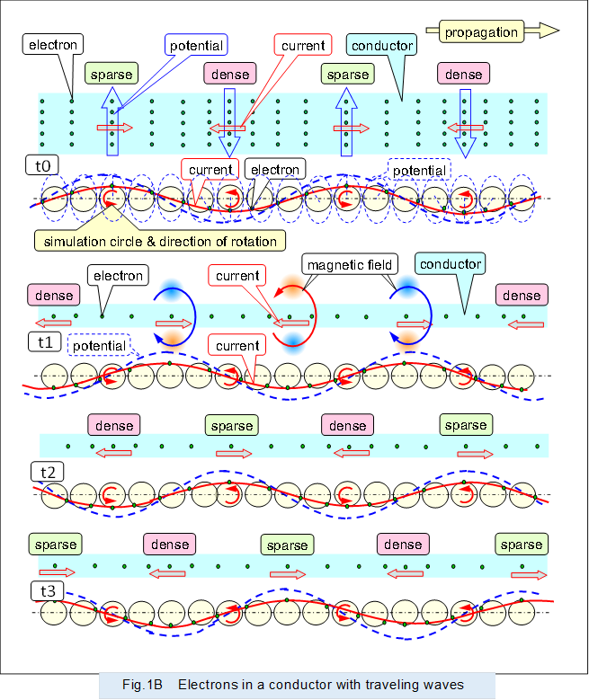The figure shows the progression of longitudinal waves (sparse and dense waves) of electrons in a conductor by moving (rotating) electrons around the circumference of the vibrating simulation circle following time at t0, t1, t2, and t3. It also shows the current and potential represented as a transverse wave. Where the electrons move faster, i.e., where the current is higher, a corresponding magnetic field is generated around the area, and it is progressing along with the current.

The current shown by the red solid line and the potential (voltage) shown by the blue dashed line are in phase.

In the figure, orange indicates the magnetic field in the direction that penetrates the screen from front to back, and blue indicates the magnetic field in the direction that penetrates the screen from back to front. The same color scheme is used below to indicate the direction of the magnetic field.

　When an electric current propagates through a conductor of small resistance, the velocity of electrons does not decay along the way. Therefore, the shape of the vibrating simulation circle is identical for each circle from upstream to downstream of the propagation.

Incidentally, when a positive current is flowing, the simulated electrons are placed on the upper side of the vibrating simulation circle, and when a negative current is flowing, the simulated electrons are placed on the lower side of the vibrating simulation circle. Then, by rotating the simulated electrons counterclockwise, the current is drawn as a natural transverse wave.

――― Supplemental vibrating simulation circle and simulated electrons ―――

For example, when a direct current (DC) of 1 [A] flows through a copper wire with a cross section of 1 [mm2], the velocity of movement (average velocity) of electrons is 0.07 [mm/sec].

Under the same conditions, with an alternating current (AC) of 1 kHz, the one-way travel distance of the reciprocating electrons is 1/2 of 0.07/1000 [mm], and the actual diameter of the vibrating simulation circle in the direction of propagation is 0.035 [µm].

This diameter is extremely small compared to the wavelength of one wavelength of 1 kHz alternating current, which is 300,000 [m].

On the other hand, the maximum value of the electrons' movement velocity is 0.07 x pi/2 (= 0.11) [mm/sec], since the maximum value of the alternating current is "pi/2 times" the average value.

Therefore, the maximum diameter in the direction perpendicular to the direction of propagation of the vibrating simulation circle, which represents the velocity of electron movement, corresponds to 0.11 [mm/sec].

（The peak value of 1.41 [A], which is the peak value of the alternating current with an effective value of 1 [A], corresponds to this 0.11 [mm/sec].）

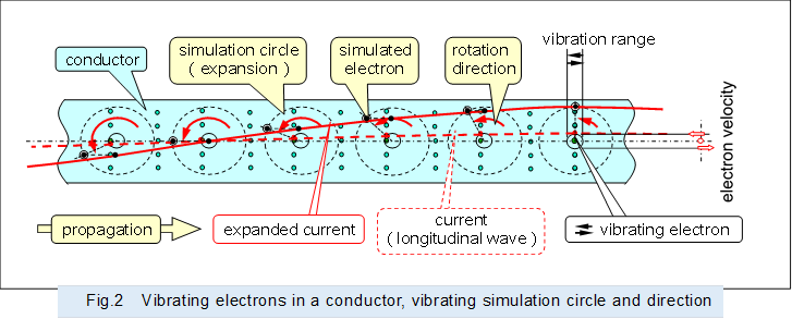
As described above, the vibration amplitude of real electrons is small, making it difficult to understand how adjacent electrons move sequentially and how their density changes. As shown in Figure 2, by placing simulated electrons corresponding to the positions of actual electrons on the circumference of an enlarged vibrating simulation circle, the amplitude of vibration is enlarged and the state of electrons becomes easier to understand.

The current shown by the red dashed line, which is difficult to understand in actual magnitude, is also shown by the red solid line with a large amplitude due to the expansion of the diameter perpendicular to the direction of propagation.

The appearance of the electrons immediately after the power supply is connected is described in "3 Propagating electrons in a conductor" below.

＜ 2  Electrons forming a standing wave type alternating current ＞

The alternating current that forms a standing wave is a longitudinal wave (sparse-dense wave) in which the sparse and dense positions are not shifted by the vibrating electrons. There are nodes and bellies: node where the electron mobility is small and the density change is large, and belly where the electron mobility is large and the density change is small.

The timing of high potential (when the electron density is at its highest or lowest) alternates with the timing of high current (when electrons move at their highest velocity in the positive or negative direction).

Figure 3 shows a simulated electron in a conductor with an alternating current flowing through it that forms a standing wave, using a vibrating simulation circle to show the magnitude of the electron's vibration, as in Figure 1 above.

Since the amplitude of vibrating electrons at each position in the standing wave is different, vibrating simulation circles of different sizes corresponding to the position are placed at each position.

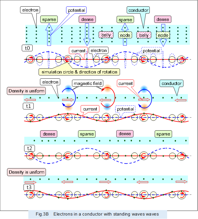As shown in the figure, the standing wave stagnates without propagating, alternating between high voltage timing (t0 and t2) and high current timing (t1 and t3).

In a standing wave, it alternates between voltage, as in potential (pressure) energy, and current, as in kinetic (velocity) energy, or paired forms, as in voltage (density energy of electrons) and current (kinetic energy of electrons). As a result, electrical energy stays in the conductor and never leaves, and power does not decay in the conductor.

＜ 3  Propagating electrons in a conductor ＞

Figure 4 shows the current, potential and electrons flowing immediately after connecting an alternating current power source to the pair of conductors.

This figure shows the electrons and current propagating from t0, before the switch is connected, to t1, t2, and t3, after the switch is connected, over time, using a vibrating simulation circle as described above.

The current propagating through the pair of conductors is a pair of longitudinal waves (sparse and dense waves), and the current and potential are symmetrical balanced signals.

In reality, it is sufficient to place the switch connected to the power supply on either the positive or negative side. However, in order to easily understand the initial state of the electrons in each conductor and their behavior immediately after connection, the switches are placed on both sides and operated simultaneously.

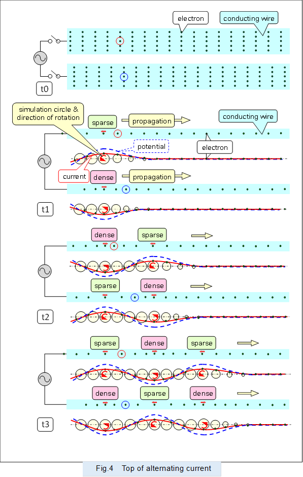Figure 5 shows how the alternating current passing through the resistor wire with electrical resistance connected to the end of the conducting wire in Figure 4 above decreases and dissipates. The current is converted into thermal energy in the resistor wire and decreases. In this figure, the vibration of electrons in the resistor wire is represented by sequentially decreasing the diameter of the vibrating simulation circle, and a series of electrons without a vibrating simulation circle is shown next to it.

The converted thermal energy heats the resistor wire, emits infrared rays, and further heats it to emit visible light, which is also the electromagnetic wave.

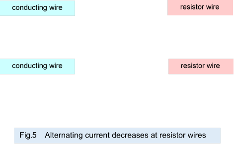
Figure 6 shows the current, potential and electrons flowing immediately after connecting a direct current power source to the pair of conductors.

The figure shows the electrons and current propagating from t0, before connecting the switch, to t1, t2, and t3, after connecting the switch, over time, in the same manner as above.

As shown in the figure, individual electrons move slowly. However, in the positive potential conductor, the leading edge of the sparse electron cluster propagates at the speed of light. And in the negative potential conductor, the leading edge of the dense electron cluster propagates at the speed of light.

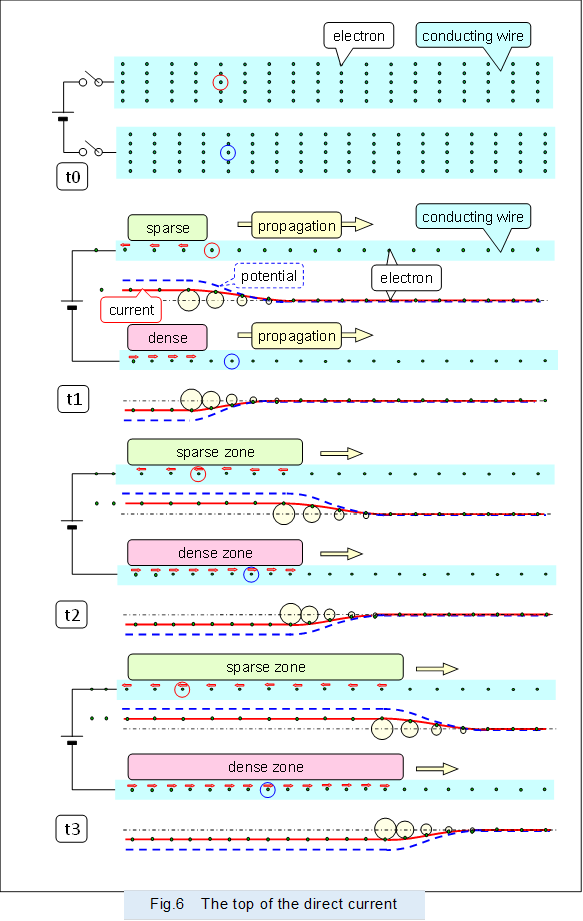To make it easier to see how the electrons stay in one place while vibrating back and forth in alternating current, or how they move slowly in the direction of propagation and power source in direct current, a red or blue circle is marked on one of the electrons in the conductors in Figure 4 and Figure 6.

＜ 4  About Transverse wave by electric field and Displacement Current ＞

As mentioned above, the current flowing through a conductor and the voltage (potential) generated there are indicators of the moving velocity and density of electrons that form longitudinal waves (sparse and dense waves). In other words, they have no substance as transverse waves.

Incidentally, waveform display devices such as oscilloscopes, for example, which are used to observe changes in current and voltage, convert the state of longitudinal waves (sparse and dense waves) caused by electrons into a transverse waveform that is easy to recognize and display.

There is no displacement current ahead of the tip where the current goes, as shown by the electrons in the conductor immediately after the power supplying as described above. Also, in the case of alternating current, if the current is dissipated in the conductor due to decrease by electric resistance, there is no displacement current beyond the point where the current is dissipated. It is described below in “Generate electromagnetic waves” that when an antenna generates electromagnetic waves, no displacement current is required because the supplied current decreases in each part of the antenna and dissipates in the antenna. And, it is described below in “Receive electromagnetic waves” that when an antenna receives electromagnetic wave, no displacement current is required because the induced currents in each part of the antenna are summed up and output.

As described above, voltage, potential, and even electric field have no entities as transverse waves. In addition, when current is supplied, there is no need to make the electrical circuit a closed loop, and no need to assume a displacement current ahead of the tip of the current that is not current. Therefore, Dr. Maxwell's equations need to be reviewed.

＜「Unclear about radio waves」・「Electrical and Magnetic forces」＞